
Introduction:
The Cox-Ingersoll-Ross (CIR) model, named after John Cox, Jonathan Ingersoll, and Stephen Ross, is a widely used mathematical model in finance for describing the evolution of interest rates. Developed in the 1980s, the CIR model has found applications in various areas such as pricing fixed-income securities, valuing interest rate derivatives, and risk management. This article aims to provide an in-depth understanding of the CIR model, its assumptions, mathematical formulation, and practical implications in financial markets.
Assumptions:
The CIR model is built upon several key assumptions:
- Interest rates are non-negative.
- Interest rates exhibit mean reversion, meaning they tend to move towards a long-term average over time.
- Interest rate volatility is proportional to the level of interest rates.
- Interest rates are continuous-time processes, meaning they can change at any point in time.
Mathematical Formulation:
The CIR model is expressed through a stochastic differential equation (SDE) that describes the dynamics of the interest rate.
Solution:
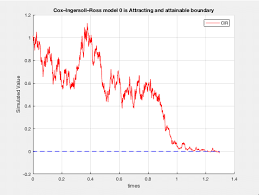
The CIR model does not have a closed-form solution like some other interest rate models. However, it can be solved numerically using techniques such as Euler’s method, Monte Carlo simulation, or finite difference methods. These numerical methods allow for the estimation of interest rate paths and the pricing of financial instruments under the CIR framework.
Applications:
The CIR model finds widespread applications in financial markets, including:
- Pricing Fixed-Income Securities: The model is used to price bonds, options, and other fixed-income securities by simulating interest rate paths and discounting future cash flows appropriately.
- Valuing Interest Rate Derivatives: Interest rate derivatives such as interest rate swaps, caps, and floors can be priced using the CIR model, enabling market participants to hedge against interest rate risk.
- Risk Management: Financial institutions use the CIR model to assess their exposure to changes in interest rates and manage interest rate risk in their portfolios effectively.
Extensions and Variations:
Over the years, researchers have developed extensions and variations of the original CIR model to better capture the complexities of interest rate dynamics. Some common extensions include the addition of jumps in interest rates, allowing for negative interest rates, and incorporating regime-switching behavior in interest rate processes.
Conclusion:
The Cox-Ingersoll-Ross model provides a valuable framework for understanding and modeling interest rate dynamics in financial markets. Its ability to capture mean reversion and volatility clustering makes it a popular choice for pricing and risk management purposes. While the model has its limitations and simplifying assumptions, it remains a foundational tool in quantitative finance, serving as the basis for more advanced interest rate models. Understanding the CIR model is essential for finance professionals and researchers seeking to analyze and navigate interest rate-related phenomena in today’s complex financial landscape.